Paper Title: Deep Residual Learning for Image Recognition
Publication Year: 2016
The Problem: As neural networks grow in depth, the effect of the vanishing/exploding gradients gets more noticeable, sometimes to the point where adding more layers yields a worse result, but not due to overfitting.
Introduction
In this paper the authors try to tackle the problem of vanishing/exploding gradients in very deep neural networks by suggesting a new architecture for neural networks. The vanishing gradients problem, simply put, is that during backpropagation each weight receives an update that is proportional to the partial derivative of the loss function with respect to that weight, and this partial derivative can be very small, especially as the network grows larger. The basic idea is to introduce an identity mapping that allows the network to skip a few layers. In theory it means that the error should not be greater than a shallow network which doesn’t suffer from vanishing gradients as much.
In More Detail
Let’s say the goal of a neural network (or part of it) is to learn some function F(x) where x are the inputs to this part of the network. The authors suggest adding a skip connection to the end, basically adding x to the output. This changes the objective function to be:
Since the change to the objective is a linear addition, the network should have no problem to learn it, and the error should not be worse than that of the network without the skip connection.
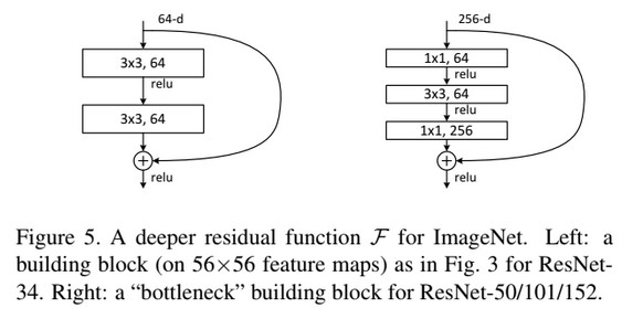
In the paper the authors suggest using an architecture made of blocks, where each block contain two or three layers, and a skip connection over the block. The following figure from the paper explains it:
Results
The authors used ImageNet as the benchmark in their experiments. Note that skip connections don’t add any more parameters to the network, so the authors could make a fair comparison for the same topology with and without the skip connections. And indeed, adding skip connections lowered the error rate on the validation set by 3%. Moreover, they managed to show that adding more layers actually improves the generalization. They used a network with 152 layers to show this point. Using this architecture they trained an ensemble to win ILSVRC’15.
Pytorch Implementation
To test the idea out I went ahead and made a basic classifier with skip connections and trained it over CIFAR10.
import torch
import torch.nn as nn
import torchvision
import torchvision.transforms as transforms
import torch.optim as optim

class ResBlock(nn.Module):
    """The ResBlock class in the paper has an increasing channel dimension for deeper layers."""
    def __init__(self):
        super().__init__()
        self.conv1 = nn.Conv2d(64, 64, 3, padding=1)
        self.conv2 = nn.Conv2d(64, 64, 3, padding=1)
    def forward(self, x):
        out = self.conv1(x)
        out = nn.functional.relu(out)
        out = self.conv2(out)
        out = nn.functional.relu(out)

        # The skip connection
        out = out + x
        return out

class ResNet(nn.Module):
    """This is a basic network with skip connections. It is different than the one suggested in the paper, and only here to show a possible implementation"""
    def __init__(self, input_channels, input_size, num_classes, blocks=5):
        super().__init__()
        self.resblocks = nn.ModuleList([ResBlock() for i in range(blocks)])
        # 1x1 convolution to make sure the channels dimension is correct
        self.channel_correct = nn.Conv2d(input_channels, 64, 1)
        self.fc = nn.Linear(input_size * 64, num_classes)
    def forward(self, x):
        x = self.channel_correct(x)
        for block in self.resblocks:
            x = block(x)
        #flatten the result, keep the batch dimension
        x = torch.flatten(x, start_dim=1)
        x = self.fc(x)
        return x

# The rest of the code is based on https://pytorch.org/tutorials/beginner/blitz/cifar10_tutorial.html

device = torch.device("cuda:0" if torch.cuda.is_available() else "cpu")
batch_size = 32
lr = 0.001
epochs = 10

transform = transforms.Compose(
    [transforms.ToTensor(),
     transforms.Normalize((0.5, 0.5, 0.5), (0.5, 0.5, 0.5))])

trainset = torchvision.datasets.CIFAR10(root='/tmp/data', train=True,
                                        download=True, transform=transform)
trainloader = torch.utils.data.DataLoader(trainset, batch_size=batch_size,
                                          shuffle=True, num_workers=2)

testset = torchvision.datasets.CIFAR10(root='/tmp/data', train=False,
                                       download=True, transform=transform)
testloader = torch.utils.data.DataLoader(testset, batch_size=batch_size,
                                         shuffle=False, num_workers=2)

classes = ('plane', 'car', 'bird', 'cat',
           'deer', 'dog', 'frog', 'horse', 'ship', 'truck')

criterion = nn.CrossEntropyLoss()
net = ResNet(3, 32*32, len(classes))
optimizer = optim.SGD(net.parameters(), lr=lr, momentum=0.9)
net.to(device)

for epoch in range(epochs):  # loop over the dataset multiple times

    running_loss = 0.0
    for i, data in enumerate(trainloader, 0):
        # get the inputs; data is a list of [inputs, labels]
        inputs, labels = data[0].to(device), data[1].to(device)

        # zero the parameter gradients
        optimizer.zero_grad()

        # forward + backward + optimize
        outputs = net(inputs)
        loss = criterion(outputs, labels)
        loss.backward()
        optimizer.step()

        # print statistics
        running_loss += loss.item()
        if i % 20 == 19:    # print every 20 mini-batches
            print('[%d, %5d] loss: %.3f' %
                  (epoch + 1, i + 1, running_loss / 20))
            running_loss = 0.0

print('Finished Training')

correct = 0
total = 0
with torch.no_grad():
    for data in testloader:
        inputs, labels = data[0].to(device), data[1].to(device)
        outputs = net(inputs)
        _, predicted = torch.max(outputs.data, 1)
        total += labels.size(0)
        correct += (predicted == labels).sum().item()

print('Accuracy of the network on the 10000 test images: %f %%' % (
    100 * correct / total))